Fluid Simulator

TLDR
There are two classic methods for fluid simulation: the Eulerian method and the Lagrangian method. This article will provide a detailed explanation of the principles and implementation of both approaches.

Comparison of Simulation Methods

Fluids typically refer to liquids or gases. Due to their similar physical properties, despite minor differences, they can share most of the same simulation methods.

In fluid simulation, we generally adopt the following assumptions:

• Incompressibility: The volume of a fluid remains essentially constant under external forces. For example, water can be considered nearly incompressible - even under a pressure of $10,000kg/cm^2$ (equivalent to the weight of a heavy truck on one square centimeter), its volume would only decrease by approximately $3\%$.

There are two classic methods for fluid simulation:

Eulerian Method

Uses a fixed grid system where each cell records fluid properties such as velocity and density. This method describes fluid behavior from a macroscopic perspective, aligning more closely with the concept of a "field," making it suitable for simulating highly continuous fluid phenomena.

Lagrangian Method

Employs a moving particle system where each particle carries fluid properties and moves with the fluid. This method tracks fluid particles from a microscopic perspective, more closely matching the natural movement characteristics of matter, making it suitable for handling free surfaces and complex boundary problems.

Eulerian Method

In the grid, we represent the velocity field with a two-dimensional vector and the density field with a scalar. Under ideal conditions, we assume the fluid has no internal friction, simplifying the computational model. In practical applications, appropriate viscosity terms are added as needed.

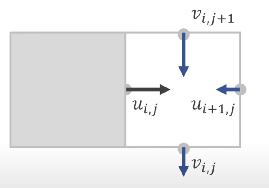
Simulating the velocity field at cell boundaries rather than cell centers is preferable, as it provides a clearer understanding of how individual cells flow into their adjacent cells.

The entire simulation process can be summarized in three steps:

1. Modify Velocity Values Based on External Forces

Here we use gravity. For all cells, $v_{i,j} = v_{i,j} + g \Delta t$, meaning we add the product of gravitational acceleration and time step to the vertical component. Gravitational acceleration $g$: $9.81 m/s^2$ Time step $\Delta t$: (e.g., $\frac{1}{30}s$)

for (let i = 0; i < gridWidth; i++) {
  for (let j = 0; j < gridHeight; j++) {
    v[i][j] = v[i][j] + g * dt;
  }
}

2. Make the Fluid Incompressible (Projection)

To maintain fluid incompressibility, we introduce the concept of divergence, which is proportional to the amount of fluid leaving a cell during a time step. In a stacked grid structure, we only need to sum the velocities of adjacent cells.

$$D = u_{i+1,j} - u_{i,j} + v_{i,j+1} - v_{i,j}$$

Physical Meaning of Divergence

• If the right side $u_{i+1,j}$ is positive, it means fluid is flowing out of this cell
• If the left side $u_{i+1,j}$ is positive, it means fluid is flowing into this cell
• If D is positive, it indicates excessive outflow
• If negative, it indicates excessive inflow
• For incompressible fluids, we need to ensure D equals 0

Force Divergence to Zero

Taking excessive inflow as an example, normally we would just flip one of the edge velocity components, but fluids cannot do this. Fluids can only push velocity components outward or pull them inward by the same amount. The solution is actually simple: distribute D evenly among the valid directional components, i.e.:

$$u_{i,j} = u_{i,j} - \frac{D}{4}$$

$$u_{i+1,j} = u_{i+1,j} + \frac{D}{4}$$

$$v_{i,j} = v_{i,j} - \frac{D}{4}$$

$$v_{i,j+1} = v_{i,j+1} + \frac{D}{4}$$

Handling Obstacles/Boundaries

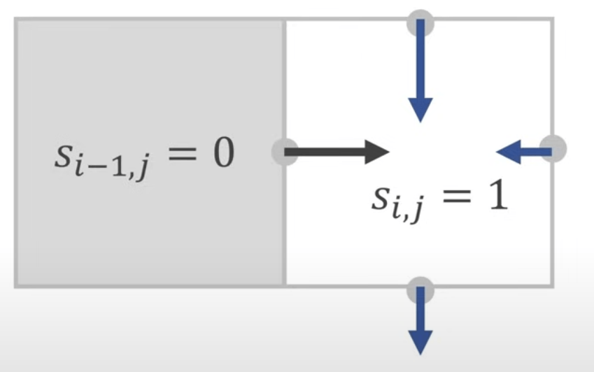
If one side is a wall or obstacle, we average the remaining edges: i.e.:

$$u_{i+1,j} = u_{i+1,j} + \frac{D}{3}$$

$$v_{i,j} = v_{i,j} - \frac{D}{3}$$

$$v_{i,j+1} = v_{i,j+1} + \frac{D}{3}$$

Typically, we store a scalar value s in each cell, setting it to 0 for obstacle cells and 1 for regular fluid cells. This value is called the Solid Fraction, representing the proportion of solid in the cell. i.e.:

$$D = u_{i+1,j} - u_{i,j} + v_{i,j+1} - v_{i,j}$$

$$S = S_{i+1,j} + S_{i,j} + S_{i,j+1} + S_{i,j}$$

$$u_{i,j} = u_{i,j} - D*\frac{S_{i,j}}{S}$$

$$u_{i+1,j} = u_{i+1,j} + D*\frac{S_{i+1,j}}{S}$$

$$v_{i,j} = v_{i,j} - D*\frac{S_{i,j}}{S}$$

$$v_{i,j+1} = v_{i,j+1} + D*\frac{S_{i,j+1}}{S}$$

We then apply this logic to the entire grid rather than individual cells. The specific method is to iterate through the grid n times, processing each cell in each iteration and applying the formulas mentioned above to make the divergence of all cells zero. This method is called the Gauss-Seidel iteration method.

for (let iteration = 0; iteration < n; iteration++) {
  for (let i = 0; i < gridWidth; i++) {
    for (let j = 0; j < gridHeight; j++) {
      const D = u[i + 1][j] - u[i][j] + v[i][j + 1] - v[i][j];
      const S = S[i + 1][j] - S[i][j] + S[i][j + 1] - S[i][j];

      u[i][j] -= D * (S[i][j] / S);
      u[i + 1][j] += D * (S[i + 1][j] / S);
      v[i][j] -= D * (S[i][j] / S);
      v[i][j + 1] += D * (S[i][j + 1] / S);
    }
  }
}

Boundary Handling

This is a very simple calculation logic. For cells at the boundary, when they access cells outside the grid, we can either treat the external cells as obstacles or copy the current cell's value.

Measuring Pressure

Fluid simulation typically requires calculating the pressure field distribution, which doesn't affect the simulation itself but provides additional information. We store a scalar pressure value in each cell, initialized to 0 $p_{i,j} = 0$. During each grid iteration, individual cells update their pressure according to the following equation:

$$p_{i,j} = p_{i,j} + \frac{d}{s} * \frac{\rho h}{\Delta t}$$

Where $d$ is the divergence, $s$ is the total number of valid cells (sum of solid fractions), $\rho$ is the fluid density, and $h$ is the cell size.

for (let i = 0; i < gridWidth; i++) {
  for (let j = 0; j < gridHeight; j++) {
    p[i][j] = 0;
  }
}

for (let iteration = 0; iteration < n; iteration++) {
  for (let i = 0; i < gridWidth; i++) {
    for (let j = 0; j < gridHeight; j++) {
      const D = u[i + 1][j] - u[i][j] + v[i][j + 1] - v[i][j];
      const S = S[i + 1][j] + S[i][j] + S[i][j + 1] + S[i][j];
      p[i][j] += (D / S) * ((rho * h) / dt);
    }
  }
}

Accelerating Gauss-Seidel Convergence with Over-Relaxation

This sounds complex but is actually quite simple. We introduce an additional constant $1<o<2$ when calculating divergence, i.e.:

$$D = o * (u_{i+1,j} - u_{i,j} + v_{i,j+1} - v_{i,j})$$

3. Moving Fluid Advection

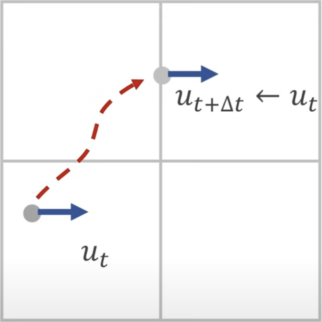
In the physical world, velocity is carried by particles in the fluid. As particles move, we attach their velocity vectors to the grid, so we need to convert particle velocities to cell velocities.

Semi-Lagrangian Method

A relatively simple and stable approach is to use the Semi-Lagrangian advection method. For example, in the figure, we want to know which fluid particle moved to the position of $u_t$?

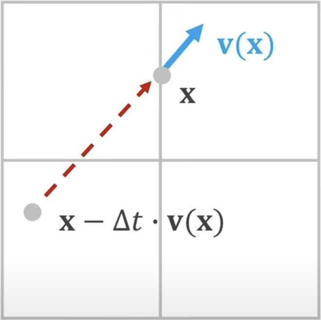
By calculating the velocity field $v(x)$ at position $x$, we can predict the position of a fluid particle one time step earlier at $x - v(x) * dt$. Since we use a straight-line path approximation, this method introduces numerical viscosity. To reduce the impact of this numerical dissipation, we can use methods like vorticity confinement to maintain fluid detail characteristics.

To calculate $v(x)$, we first need to compute the vertical component $\bar{v}$ and horizontal component $u_{i,j}$. $\bar{v}$ can be simply calculated by averaging the $v$ values in the neighborhood:

$$\bar{v} = \frac{v_{i,j} + v_{i,j+1} + v_{i-1,j} + v_{i-1,j+1}}{4}$$

To calculate $\bar{v}$ at any position, we need to introduce weighted averaging:

$$\bar{v} = w_{00}w_{10}v_{i,j}+w_{01}w_{10}v_{i+1,j}+w_{01}w_{11}v_{i,j+1}+w_{011}w_{11}v_{i+1,j+1}$$

Smoke Advection

Visualization Effect

This is only for additional display effects and does not affect fluid simulation calculations.

We can add a density value between 0 and 1 based on the velocity field already stored in each cell, stored at the center of each cell. To calculate the new density value in a cell, we use the velocity field value at the cell's center, then step back one time step and interpolate the density at the previous position.

Streamline Visualization

Streamline visualization is also simple. At the base position $x$, we sample the velocity field, then update $x$ through $s*v$.

Demo

Lagrangian Method

In the previous section, we introduced the basic concepts of the Lagrangian method. This approach simulates fluid behavior by tracking the motion of each particle from a microscopic perspective. While this method is very intuitive (for example, we can imagine simulating water flow by tracking each water molecule's movement), it faces significant computational challenges in practical applications. For instance, even 1 cubic centimeter of water contains trillions of water molecules, making it impractical to directly track each molecule's movement.

SPH (Smoothed Particle Hydrodynamics)

To maintain the advantages of the Lagrangian method while addressing computational complexity, we introduce the SPH (Smoothed Particle Hydrodynamics) method. The core idea of SPH is to treat each particle as a "fuzzy" particle with a smoothing radius rather than a precise point. Specifically:

• Each particle has a circular influence range with radius $R$
• Within this range, the particle's influence gradually weakens from center to edge
• This allows us to simulate overall fluid behavior with relatively few particles
• While maintaining fluid continuity and smoothness

In SPH, each particle carries a density field that describes its influence on the surrounding space. By superimposing the density fields of all particles, we obtain the density distribution of the entire fluid. This density field-based description enables more accurate simulation of fluid physical properties.

Smoothing Function

To describe this smooth particle influence, we need to define a smoothing function. The simplest smoothing function is linear:

$$y(influence) = \begin{cases} R - x(distance) & \text{if } -r \leq x \leq r \\ 0 & \text{otherwise} \end{cases}$$

However, this function is not smooth enough at both edges and center, resulting in a density field that doesn't transition continuously. Therefore, we can use more complex smoothing functions, such as:

$$y(influence) = \begin{cases} (r^2 - x^2)^3 & \text{if } -r \leq x \leq r \\ 0 & \text{otherwise} \end{cases}$$

Density Field and Pressure

From our previous discussion of the Eulerian method, we know that fluids are incompressible. This means:

1. Particles always move from high-density to low-density regions
2. This movement continuously attempts to correct overall density differences
3. This is essentially a gradient operation, where we constantly seek the direction of maximum density gradient
4. Particles move along this direction until reaching equilibrium

In a fluid initialization scenario:

• We introduce multiple particles and apply gravity
• Particles fall under gravity
• They begin to diffuse and escape under the influence of other particles' density fields
• Pressure can be expressed as: $p = (density - targetDensity) * pressureMultiplier;$
  • Where $pressureMultiplier$ is the specified pressure coefficient

Improvement of Smoothing Function

During the process of escaping other density fields, for a single particle's density field, the acceleration of sampling point movement matches the slope of our defined smoothing function. However, the previously used smoothing function has an issue:

• When sampling points are very close to the particle
• Because the slope of the smoothing function at X-axis 0 is almost 0
• This causes sampling points that should escape the particle to become stationary

To solve this problem, we need to update the smoothing function:

Additionally, a paper points out that in Lagrangian fluid simulation, particles tend to get too close to each other. They introduced the concept of near pressure by making the smoothing function sharper to increase pressure when particles get too close, enhancing the tendency for particles to escape.

Pressure Calculation Optimization

Application of Newton's Third Law

According to Newton's Third Law, every action has an equal and opposite reaction. In fluid simulation:

• When a particle experiences pressure from other particles
• It also exerts an equal and opposite pressure on other particles
• To simplify calculations, we can use a shared pressure approach:
  • Use the average of the target particle and sampling point pressures
  • Instead of the original pressure value calculated directly from the target particle

Performance Optimization

After solving the above problems, to calculate the true escape direction and velocity of the current sampling point, we need to perform a weighted sum of all particle density fields. Within a single time step, we perform the following operations:

function simulationStep(deltaTime) {
  // apply gravity and calculate density
  parallel.forEach((p, i) => {
    velocities[i].y += Gravity * deltaTime;
    densities[i] = CalculateDensity(positions[i]);
  });

  // calculate and apply pressure forces
  parallel.forEach((p, i) => {
    const pressureForce = CalculatePressureForce(positions[i]);
    // F=ma => a=F/m
    pressureAcceleration = pressureForce / densities[i];
    velocities[i] += pressureAcceleration * deltaTime;
  });

  // update positions and resolve collisions
  parallel.forEach((p, i) => {
    positions[i] += velocities[i] * deltaTime;
    ResolveCollisions(positions[i], velocities[i]);
  });
}

This clearly imposes a significant performance burden. For a single particle, we need to loop through all other remaining particles and calculate pressure based on the density field. In reality, it's easy to see that we only need to calculate other particles within the sampling radius of a single particle.

Spatial Lookup

We can divide the canvas into a grid where each grid's side length equals the sampling radius. For a single particle, we only need to focus on particles in the 9 surrounding grids centered on the particle's grid. For any grid, it stores a list of particles currently located in that grid, and this list continuously updates its particle elements as the fluid simulation progresses. Since the space is divided into independent grids without dependencies, CUDA acceleration could be introduced here. However, since we're currently only considering JS-based visualization effects, we'll stick with the CPU-computed version.

Performance Optimization Direction

WebGPU might be a good direction for performance optimization, but since I'm not very familiar with it yet, we'll set this aside for now.

For a single grid, we represent it through rows and columns. However, we can store each grid's particle list using a spatial hash table, allowing us to quickly find the grid containing a particle through the hash table's key. For example, for grid coordinates $x,y$, we can use $key = x * P_1 + y * P_2$ as the hash table's key, where $P_1,P_2$ are two arbitrary prime numbers. After calculating all particles' corresponding keys, we can perform a simple incremental sort, making particles in the same grid adjacent in the array, enabling efficient and fast iteration.

In addition to the particle hash table, we need to maintain a hash index table that maps to the index position in the particle hash table where we can find the corresponding particles when we locate a specific grid.

However, since different grids might yield the same hash key, we also need to perform distance calculations to exclude grids beyond the 9 surrounding grids that might match the hash value.

Demo

Interaction Instructions

You can attract fluid with the left mouse button and repel fluid with the right mouse button to observe the effects of Lagrangian fluid simulation.